NeRF -- From Foam Guns to Red Drums

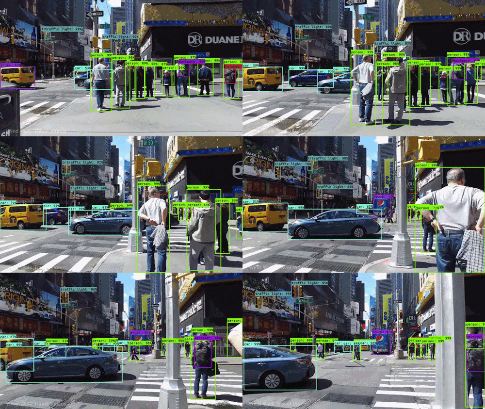
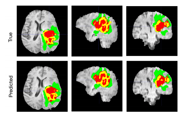
08 Dec 2021 | computer vision machine learning volumetric rendering Ocejo, Clemente

Computer vision is an exciting domain within machine learning and has applications to some of the most high-stakes problems such as autonomous vehicles, military defense, and medical imaging tasks.

Okay I will admit, the last GIF is not actually real but it’s pretty good (or bad).In many of these tasks it is super useful to develop algorithms for generating 3D models from 2D images to gain a better representation of our world. A popular family of methods for this that has gained traction in recent years is called neural volume rendering. These methods have seen such popularity partly due to the impressive results of the NeRF paper by Mildenhall et al. So let’s check out exactly what’s so cool about it!

Before diving straight into the details I want to highlight some of the work leading up to NeRF to give some context of the field during the time and highlight some of the important contributions.

One model preceding NeRF was the DeepSDF model which used a DNN (Deep Neural Network) to model the SDF (Signed Distance Function) of the object in the image in order to generate a 3D representation. This is done through an MLP consisting of 8 layers with 512 hidden units each and ReLU activation functions. Tanh is used to generate the final output estimating the SDF. While this is able to generate some pretty impressive results, you may have noticed that this is not accomplishing something as amazing as what I described in the intro. For DeepSDF to work effectively, you need a 3D dataset where you have access to the SDF values in order to train it. This was a key motivator for NeRF along some other things that I will cover later.

NeRF is able to impressively generate new realistic 3D views of a scene given many different views of the same scene. This allows you to generate a realistic model of the scence which is invaluable in computer vision. NeRF is also able to do this without access to the ground-truth geometries necessary for something like regressing on the signed distance function.

At a high level, NeRF is able to create compelling 3D scenes from 2D images through the following approach:

1. Sample a set of 3D points by marching camera rays through the 2D scene
2. Use the generated 3D points along with the 2D angle vector of the camera view as input to the neural network
3. Accumulate predicted colors and densities into a 2D image of a new view using classical volume rendering techniques

You can then easily apply gradient descent to minimize the error between our input images and their corresponding NeRF reconstructions.

One of the primary advantages of NeRF is that it is able to render these new scene views with only 2D images as input. NeRF does this by utilizing a key fact about a common technique known as volume rendering, which is that it is easily differentiable.

Volume rendering is a technique which allows you to generate a 2D rendering of a scene given the coloring and alpha of the points along rays in the scene. This is where the idea of ray marching comes into play. NeRF utilizes the ray rendering technique to optimize itself based on input images.

NeRF first generates the points along rays of this scene by simply marching through an assumed bounding box containing the scene. These points are then collected along with camera views and fed into an MLP which is to predict the color and volume density of each point along the ray. You may already see how this is useful in our original task having mentioned volume rendering.

An interesting thing to notice about the MLP used in the NeRF model is that it is very similar to the one found in the DeepSDF model. It also consists of 8 layers, this time with 256 hidden units each, using ReLU activation functions. However, NeRF does not utilize the full input across all layers and adds an additional hidden layer. The first 8 layers only attend to the 3D coordinate of the input image. These layers in charge of outputting the volume density in order to accurately reflect the fact that this is not dependent on the view angle from the camera. They also output a 256 dimensional hidden vector which is concatenated with the viewing directions in order to produce the RGB color which could be impacted by the camera view due to lighting effects.

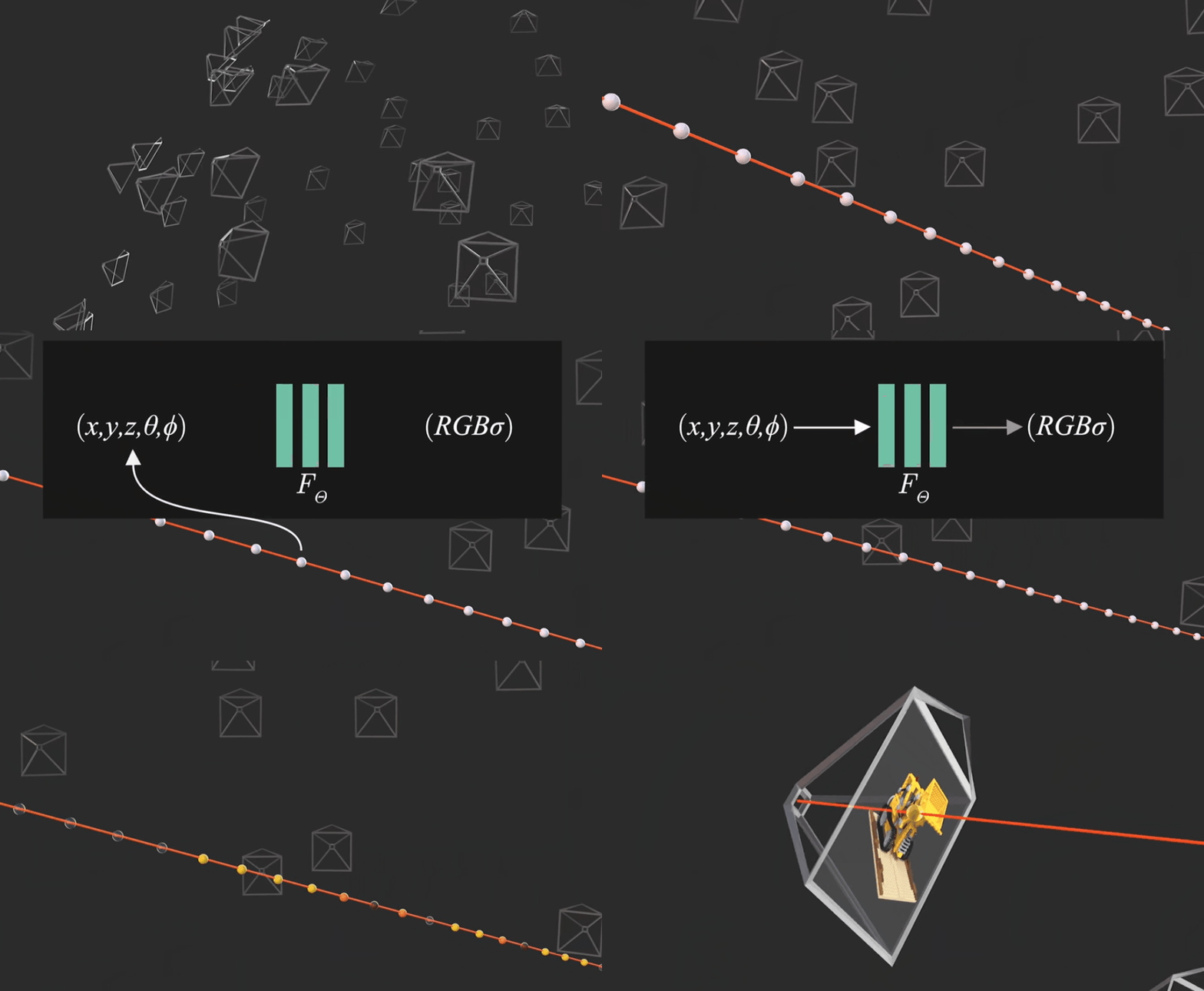
After producing these 2 (or rather 4 output values since the color is an RGB value) NeRF must then render an image that we can compare our input with in order to generate a loss to back propogate over. As mentioned earlier, this can thankfully done through classic techniques which are easily differentiable. The way the expected color of the camera ray is calculated is with the following equation:

\[\begin{equation} C(r) = \int_s^fT(t)\sigma(r(t))c(r(t), d)dt \\ T(t) = \exp(-\int_s^t \sigma(r(s))ds) \end{equation}\]

In this equation the function T(t) represents the probability that the ray travels the entire path across the scene without colliding with any other particle. This makes sense since the volume density can intuitively be thought of as the probability of a ray ending at the point. You can think of this whole process as projecting a ray out from our eye into the scene and coloring a canvas located somewhere between the two with the first color we see similar to in ray tracing.

Another key innovation that NeRF came with was the resolution at which it is able to generate new views of scene. Work on scene representation networks by Stizman was unable to produce multi-view consitent scnes and cannot represent details very well. Local light fusion fields by Mildenhall et al. improve this inconsistenty tremendously but cause flickering artifacts. Lombardi was able to produce much smoother scene representations but are not able to produce the high-resoultion scenes that NeRF can as seen below.

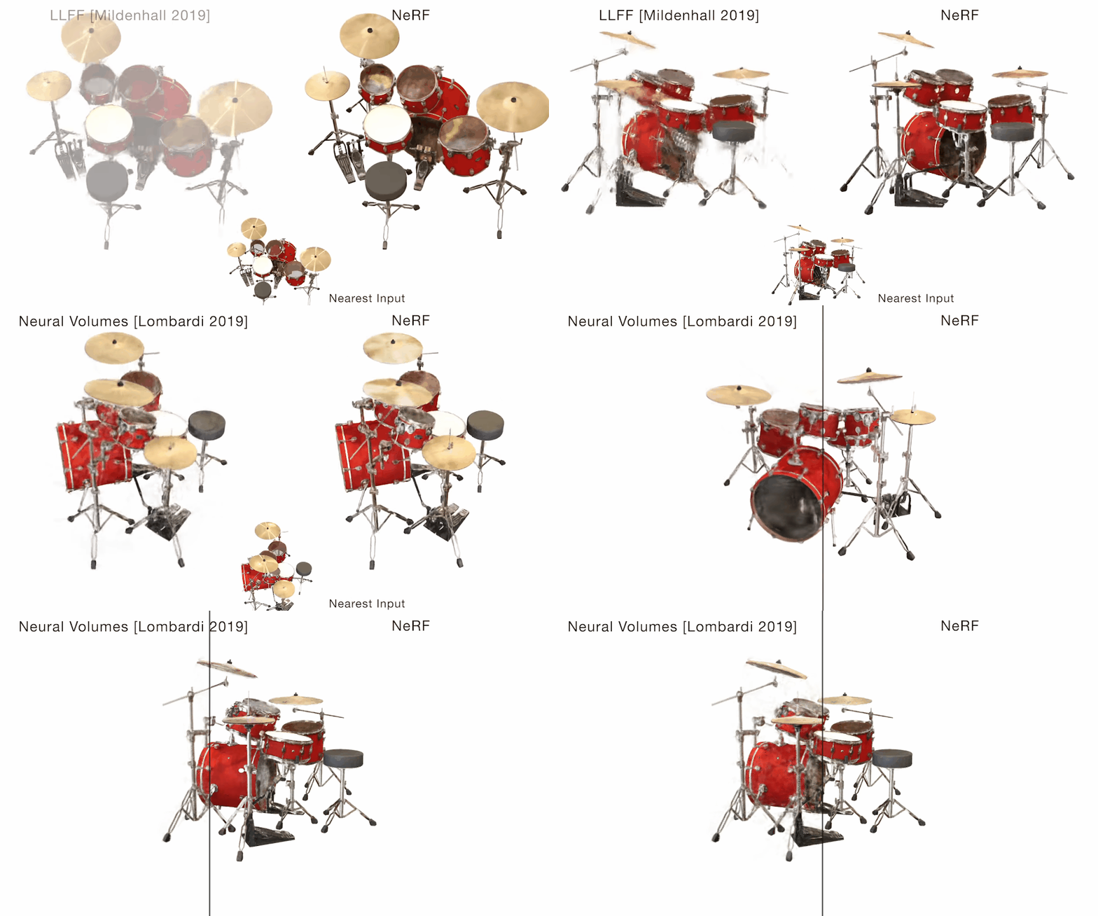
NeRF was able to achieve such high resolution through a modification in their integral numerical estimation technique. Quadrature is often used to accomplish such estimations but in the context of rendering this is often done via deterministic quadrature. This would limit the locations queried by the MLP to a discrete set which limits the output resolution potential. NeRF circumvents this by using a stratified sampling approach where they partition the scene bounds into evenly spaced bins and sample uniformly from them. The whole estimation can be formalized as follows:

\[\begin{equation} \hat{C}(r) = \sum_{i=1}^NT_i(1-\exp(-\sigma_i\delta_i))c_i \\ T(t) = \exp(-\sum_{j=1}^{i-1} \sigma_j\delta_j) \end{equation}\]

Since this equation is easily differentiable, NeRF is able to attach the rendering method directly onto the MLP pipeline and train the two together as an end-to-end model using the loss from the generated rendered view and the input image.

While the model I have described already produced promising results, there were additional optimizations made to the underlying NeRF model to achieve state-of-the-art performance.

Instead of inputting the 3D coordinate and 2D camera view into the model directly, NeRF first maps these to a higher dimensional space in order to aid the representation of high-frequency variation in color and geometry. To do this they borrow a mechanism from the Transformer architecture which is referred to as the positional encoding. They use the cyclical properties of sin and cos to create a function that passes the input coordinates through alternating sin and cos functions at each dimension to generate the desired dimensional output. This is done independently for each three coordinates in the 3D position vector to output a 10 dimensional representation. This also done independently on the three coordinates of the unit viewing vector generated from the camera view angles to output a 4 dimensional representation.

Another optimization is performed on the ray marching technique used to sample the N points being used to generate neural radiance fields. By simply sampling N points over the entire ray without an heuristic information, we risk repeatedly sampling free space and occluded regions which do not contribute to the rendered image. To do this NeRF creates a hierarchical model pipeline by introducing a “fine” network to reinforce the “coarse” network that makes the initial prediction. More formally the ray color output from the “coarse” network is taken and rewritten to be a weighted sum of the sampled colors on the ray as follows:

\[\begin{equation} \hat{C_c}(r) = \sum_{i=1}^{N_c}w_ic_i \\ w_i = T_i(1-\exp(-\sigma_i\delta_i)) \end{equation}\]

These weights are then normalized to produce a piecewise-constant PDF along the ray. Using this informed PDF we generated from the weights, NeRF can sample a second set of locations to use in the “fine” network. This “fine” network then does the same thing as the “coarse” network but on the initial set of points as well as the new informed set of points of the same size.

These two optimizations together allow for NeRF to generate the high-resolution views that it is able to from 2D images.

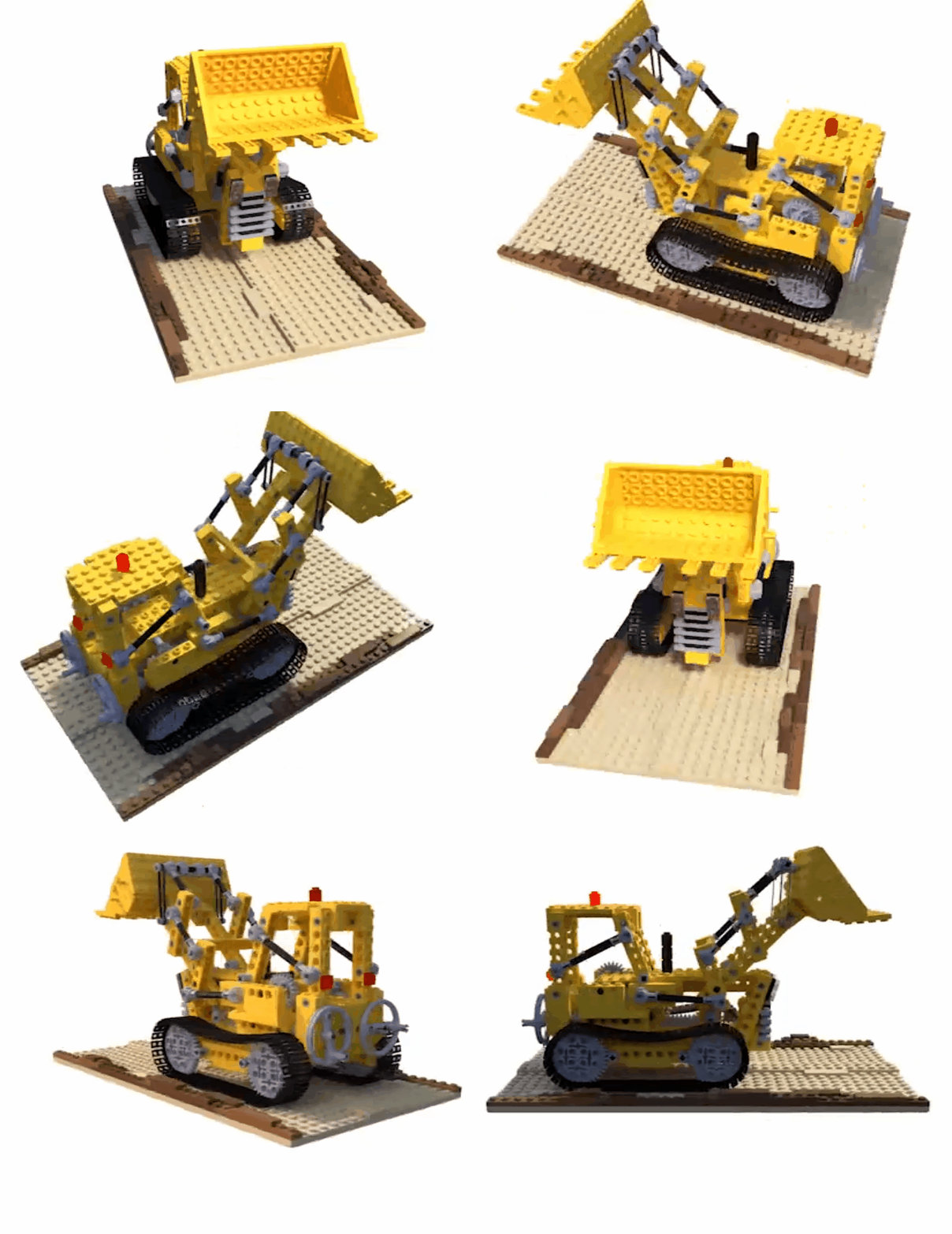
A cool experiment is taking a look at the result of training a simple NeRF model with only position coordinates (no camera view) and only a single network (no hierarchical coarse then fine network) on the bulldozer scene I showed earlier as compared to the full network on the scene.

So let me just quickly summarize why NeRF is so cool:

1. It allows for new view renderings of complex geometric shapes given 2D input images where as some previous models could overcome the 3D ground-truth requirement for only simply geometries.

2. Produces very high-resolution scenes through clever continous encoding of volume features when compared to models using volumetric representations.

3. It does all of this with a really simple model that you can fire up in 50 lines on google colab.

Hopefully this post gave you a little insight on the world of scene representation and made you love NeRF as much as I do!